Functions with pretensions - Solution
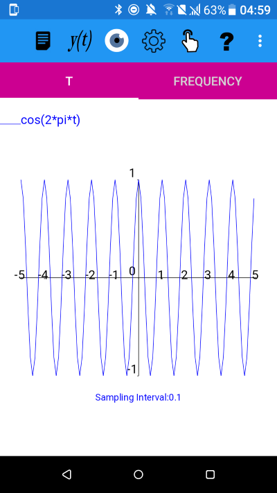
The function y=cos(2*pi*t) with -5<=t<5 and a sampling interval of 0.1
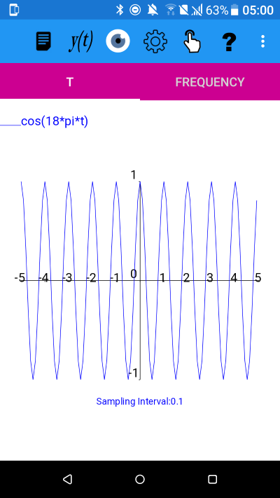
The function y=cos(18*pi*t) with -5<=t<5 and a sampling interval of 0.1
The two graphs look exactly the same.
Aliasing and the Sampling Theorem
The sampling theorem states that the sampling interval must be less than or equal to Tn=1/(2*f) seconds (Tn is the Nyquist Interval) in order to be able to correctly represent a frequency of f Hz. If the signal is sampled with a sampling interval below the Nyquist interval then the digital representation of the signal will exhibit aliasing.The Nyquist (or folding) Frequency
An equivalent test to the sampling theorem is to compare the signal frequency to the Nyquist frequency.The Nyquist Frequency, Fn, i.e. the highest frequency that can be correctly represented at a sampling frequency of fs, is given by
Fn = fs/2 where
fs is the sampling frequency (or sampling rate) and
fs = 1/(sampling interval)
Where frequencies in the signal are greater than the Nyquist frequency, aliasing will occur, i.e. the higher frequencies will fold into lower frequencies.
The Aliasing Frequency
Supposing we have a signal of single frequency, f, which has been sampled such that Fn, the Nyquist Frequency is less than the signal frequency, f. What is the folding or aliasing frequency of the signal, i.e. what frequency will the digital representation appear to be at?To find the aliasing frequency, divide the sampling frequency by the signal frequency and express the result to the nearest integer. i.e. fi=round(fs/f)
The signal will alias to Falias = Absolute((fs*fi) - f)
Why do our two plots look the same?
The second plot of y=cos(18*pi*t) with a sampling interval of 0.1 exhibits aliasing. The original function has a frequency, f= 9
The sampling theorem states that the sampling interval needs to be less than or equal to 1/(2*9) i.e. less than approximately 0.0555555 in order to correctly represent the frequency of the signal. As our sampling interval is too large (or equivalently the sampling frequency is too small) then we expect aliasing.
The sampling frequency fs is the reciprocal of the sampling interval i.e. fs = 1/(0.1)=10.
The aliasing frequency is found by considering fi=round(fs/f) = round(10/9)=1
and the sampled signal will alias to;
Falias = Absolute((fs*fi) - f) = abs(10*1-9)=1
So y=cos(18*pi*t), i.e. a frequency of 9, at a sample interval of 0.1, aliases to y=cos(2*pi*t) i.e. a frequency of 1, and that is why the two graphs look the same.
Correctly representing cos(18*pi*t)
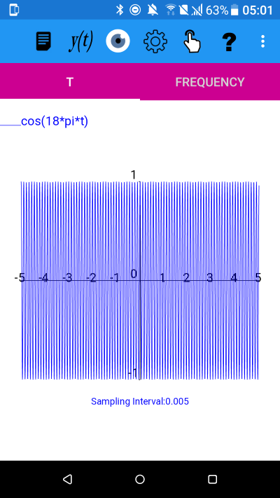
To preserve the correct frequency of y=cos(18*pi*t) we need to use a sampling interval which is less than the Nyquist interval 1/(2*9) = approx 0.0555555. Below is the graph with a sampling interval of 0.005 and the sampled function is no longer pretending to be something that it isn't!The function y=cos(18*pi*t) with -5<=t<5 and a sampling interval of 0.005
plotXpose app is available on Google Play and App Store
Google Play and the Google Play logo are trademarks of Google LLC.
A version will shortly be available for Windows.
A version will shortly be available for Windows.
plotXpose app is a companion to the book Mathematics for Electrical Engineering and Computing by Mary Attenborough, published by Newnes, 2003.


